Math 1B  Chapter 7 Test  fall ’06             Name________________________

Show your work for credit.  Write responses on separate paper. Do not abuse a calculator.

 

1.      Suppose a quantity P satisfies the differential equation .

a.       Find the equilibrium solutions for P and classify each as either stable or unstable.

b.      At what value of P is P increasing most rapidly?

2.      Consider the initial value problem .

a.       Solve for x as a function of t using the method of separating variables.
Note: You may need to use integration by parts.  If you do, show the table of u,v,du,dv expressions.  Do not rely on a calculator to get the result.

b.      Use Euler’s method with a step size of 0.25 to get a numerical approximation for .  Show your calculations by completing the table below:

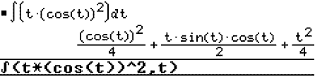
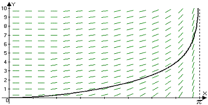
3.      Consider the family of functions defined by .  Find the family of orthogonal trajectories.

year	Population
1960	11209160
1970	14598316
1980	17848320
1990	20278957
2000	22191087
2005	23070170

4.      Consider the table below which tabulates the population of Taiwan in various years:

a.       Fit a natural growth model to the populations in years 1960 and 1970.  How well does the model predict the projected population for 2005? 

b.      It appears the growth rate may have reached a maximum in the year 1970.  Assuming that is true, write a logistic differential equation for the population of Taiwan.  Specify plausible values for both r and K.
 

5.      Solve the initial value problem: .

6.      Suppose that a spherical raindrop is evaporating as it falls so that its mass is decreasing at a rate proportional to its surface area.  That is, .  Substitute  (where  is the mass density of water and r is the radius of the spherical raindrop) to show that .

7.      Human and mosquito populations in a swampy equatorial environment are modeled by the system of differential equations,     
                                            . 

a.       Combine these equations to get a separable differential equation in M and H and Show that there exists a constant A such that .  What is the value of A if at some time there are 10 humans and 1000 mosquitos?

b.      Is one or the other of these population dependent upon the other for their survival? 
Why or why not?

 

 

Math 1B  Chapter 7 Test Solutions  fall ’06

 

1.      Suppose a quantity P satisfies the differential equation .

a.       Find the equilibrium solutions for P and classify each as either stable or unstable.

The zero at  is unstable.  The zero at P = 100 is stable. 

b.      At what value of P is P increasing most rapidly?
The maximum for  occurs at the vertex, which is halfway between the two zeros:

2.      Consider the initial value problem .

a.       Solve for x as a function of t using the method of separating variables.


It’s interesting to compare this result with the TI-89 result:

and verify that they differ by a constant. 

Do determine the constant will satisfy the initial condition, plug in t = 0  and x =  :  .  Now, solving for x we have  

b.      Use Euler’s method with a step size of 0.25 to get a numerical approximation for .  Show your calculations by completing the table below:
 

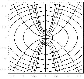
3. Consider the family of functions defined by
   
   .  Find the family of orthogonal trajectories.
   
   
   
    means that for the orthogonal trajectory,
   
   .  Now, in the original equation,
   
   .  Substituting this into the equation for the orthogonal trajectory we can solve for y by separating variables:
   
   
   In Mathematica, you could draw these curves like so:
   

To be sure, this may not be the best approach to plotting the orthogonal trajectories.  In Multivariate Calculus (Math 2A at COD) you’ll learn about contour plots.  Here are the commands for using contour plots to show these orthogonal trajectories:

c1 = ContourPlot[y/(1+x^2), {x,-8,8},{y,-8,8},ContourShading → False, PlotPoints → {245,245}]; c2 = ContourPlot[y^2+x^2/2+Log[Abs[x]], {x,-8,8},{y,-8,8},ContourShading → False, PlotPoints → {245,245}]; and then Show[c1,c2];

 

year	Population
1960	11209160
1970	14598316
1980	17848320
1990	20278957
2000	22191087
2005	23070170

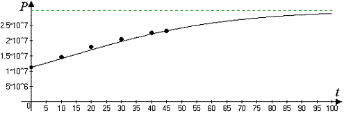
4.      Consider the table below which tabulates the population of Taiwan in various years:

a.       Fit a natural growth model to the populations in years 1960 and 1970.  How well does the model predict the projected population for 2005? 

Let t be the years since 1960 then .  To find r,  plug in the 1970 data:
Thus,

b.      It appears the growth rate may have reached a maximum in the year 1970.  Assuming that is true, write a logistic differential equation for the population of Taiwan.  Specify plausible values for both r and K.

If  is maximal in 1970, then the carrying capacity would be 2*(14598316) = 29196632 and the logistic model would look like this  - forgive the over-stated accuracy.   We’ll round to three digits so as not to seem utterly ridiculous.  This ODE is solved by separating variables in the usual way:
 .  At this stage we say that when t = 0, .  Solving for P  yields  
It remains to approximate r.  We have 4 data after 1870 we could use.  How about the most distant? When t = 45 (2005) we have  So  Below is a plot of this function over the tabulated data.

5. Solve the initial value problem:
   
   .
   
   
    
   where u = 1 + sin x .  Substituting v = e^y + 1 in the first yields the following:
   
   
   
   .  This is as good a time as any to π impose the initial conditions and solve for c: 
   
   .  Thus,
   
   
   
6. Suppose that a spherical raindrop is evaporating as it falls so that its mass is decreasing at a rate proportional to its surface area.  That is,
   
   .  Substitute
   
    (where
   
    is the mass density of water and r is the radius of the spherical raindrop) to show that
   
   .
   Substituting
   
    into
   
    yields
   
   
   
   

7.      Human and mosquito populations in a swampy equatorial environment are modeled by the system of differential equations,     
                                            . 

a.         Separating variables:



 
 
If H = 10, M = 1000,

b.      According to the model, in the absence of mosquitoes the human population will grow at a relative growth rate of 1%, while the mosquitoes, in the absence of humans will grow at a relative growth rate of 20% - go mosquitoes!

 

As an afterthought, one might be interested in how to plot the solution curves for various initial populations.  In Mathematica, you could use the ImplicitPlot feature in the Graphics subdirectory of the StandardPackages in Addons.  To do this, you type (note “`” back single quote usage on “~” key):

<<Graphics`
After quite a bit of fiddling, I arrived at the following command that plots part of the solution curve for this problem:

ImplicitPlot[(x*Exp[-0.002*x])/(y^20*Exp[0.04*y^2]) → 2.47875*^-20,{x,1,8000},{y,1,30}, PlotRegion → {{0,1},{0,1}},AspectRatio → .618, AspectRatioFixed → False]

This produces the graph below: 

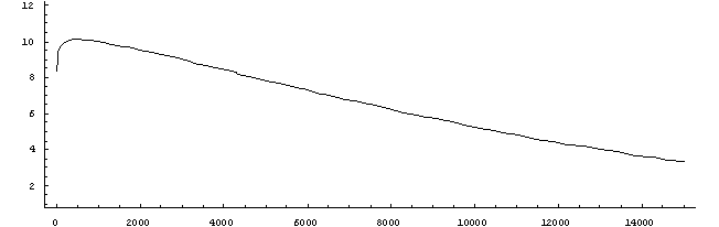
Looks like the mosquitoes thrive and the people dwindle.