Math 1B 5.4#24

 

The Fresnel integral functions (sometimes called Fourier Cosine and Fourier Sine integral functions) are

You can plot these on the TI-89/200, but it’s truly a brutal and lengthy process for the poor things, taking maybe 7 hours and likely exhausting your batteries if they don’t start fully charged. 

 

We could do something like the following on the TI-89/92/200, and produce almost exactly the same graph in a few seconds, but I’m going to use the software MATLAB, (available on computers at COD) to illustrate some of its syntax.

 

Start by creating a relatively fine partition of [0,8] with 7999 evenly spaced interior points (8000 subintervals and 8001 points, all together including the endpoints.) 

 

>> t=0:0.001:8;

 

At this stage, t is the vector of 8001 values,

 

t = [0, 0.001, 0.002, 0.003, … , 7.999,8]. 

 

We can use that now to create a vector of 8001 values on this domain:

 

>> I = sin(pi*t.^2/2);

 

The “period” symbol here indicates that, rather than squaring the entire vector, we want to square each element of the vector. 

 

To check what’s up, try looking at a few elements of I:

 

>> I(1)

ans =

  0

I(1) is the first element of the I vector and which evaluates  at the first element of the t vector, which is 0.  So this shows that sin(pi*0^2/2) = sin(0) = 0, as it should.  Similarly I(1001) is the gives the value where t = 1:

 

>> I(1001)

ans =

     1

 

In MATLAB we can then easily create a vector of 8000 partial right hand Riemann sums,  by multiplying each term by  (or, equivalently, dividing each term by 1000) and then using the cumsum to create a vector of 8001 cummulative sums up to and including the n^th element of the vector:

 

>> S = cumsum(I/1000);

 

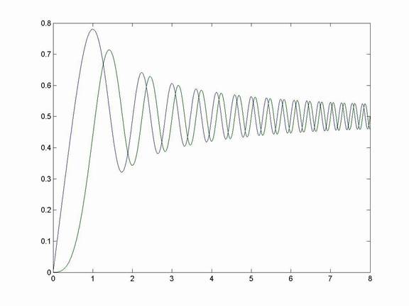
This is the sequence of  S(x) values we want to plot.  Before we do, let’s also repeat all this for the Fresnel cosine integral function:

 

>> J = cos(pi*t.^2/2);

>> C = cumsum(J/1000);

>> plot(t,C,t,S)

 

 

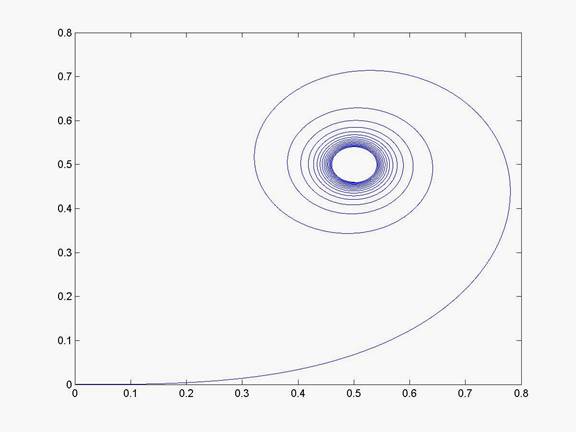
One more thing before we leave MATLAB for now.  If we plot S against C we can an interesting shape called the Cornu spiral:

 

>> plot(C,S)

 

Ok, now to answer the questions in the text. 

 

(a)    S(x) will have local maxima where the integrand switches from a region of positive values (where the integral’s area is increasing) to a region of negative values (where the integral’s area function is decreasing.)  This is where , where k is any integer.  That is, the input is an odd multiple of pi.  Solving for t we have .

(b)   The inflection points occur where the integrand achieves a max (a min.)  These are the points where the area stops increasing (decreasing) at an increasing rate and starts increasing (decreasing) at a decreasing rate.  For S(x), this is where  where   On MATLAB,
>> S(1001)
ans =
    0.4388
So the function is concave up on (0,0.438)  where else?

(c)    I can use guess and check to solve  for x.
>> S(800)
ans =
    0.2489
>> S(701)
ans =
    0.1725
>> S(751)
ans =
    0.2093

(d)    I’d say there is a horizontal asymptote, but I’ll leave it to you say why.